Physics
Physical Validity of the Mesh Current Method
An independent study showing that the mesh current method, a standard technique for analyzing planar circuits, follows directly from charge and energy conservation, verified on two- and three-mesh circuits with three independent methods.
- independent methods gave identical branch currents
- 3 of 3
- net current in R₂ of Circuit B, from mesh currents of 4 A and 3 A
- 1 A
- Field
- Physics
- Researchers
- Siwoo Kim
- Updated
- October 2026
Overview
The mesh current method is usually taught as a recipe: assign a circulating current to each mesh, write a voltage equation for each loop, and solve. Because no single mesh current can be measured in a branch shared by two meshes, this independent study asks whether the method is a physically valid description of a circuit or only a bookkeeping device.
Theoretical Background
- Kirchhoff's current law (KCL) expresses conservation of charge: in a steady state, charge cannot accumulate at a node
- Kirchhoff's voltage law (KVL) expresses conservation of energy: a charge carried around a closed loop returns to its starting potential
- Both hold under the lumped-element approximation, so any method logically equivalent to them inherits their physical validity
Derivation
- In a planar circuit with b branches and n nodes, only n − 1 node equations are independent, leaving b − (n − 1) independent loop equations, which equals the number of meshes m
- When each branch current is written as the sum of the mesh currents through it, every mesh current enters and leaves each node it touches, so KCL holds identically for any mesh-current values
- KVL around each mesh then gives exactly m equations for m unknowns: charge conservation is built in by construction, and energy conservation is enforced explicitly
Why no physical constraint is lost
1
Branch currents
b unknowns, with KCL at nodes and KVL around loops
2
Mesh currents
Write every branch current as a sum of mesh currents
3
KCL by construction
Each mesh current enters and leaves every node it touches
4
KVL per mesh
m equations for m unknowns, with m = b − (n − 1)
Numerical Verification
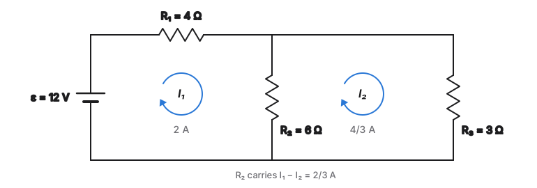
- Circuit A (two meshes): a 12 V source with R₁ = 4 Ω, a shared R₂ = 6 Ω, and R₃ = 3 Ω
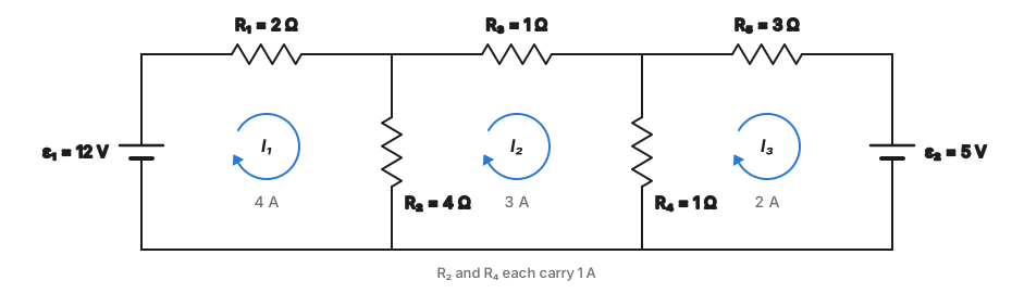
- Circuit B (three meshes): sources of 12 V and 5 V with R₁ = 2 Ω, R₃ = 1 Ω, and R₅ = 3 Ω, plus R₂ = 4 Ω shared by meshes 1 and 2 and R₄ = 1 Ω shared by meshes 2 and 3
- Each circuit was solved three ways: the mesh current method, direct branch-current analysis with the full set of Kirchhoff equations, and circuit simulation
Circuit A · two meshes
Circuit B · three meshes
Results
- Circuit A: I₁ = 2 A and I₂ = 4/3 A, so the shared resistor carries 2/3 A
- Circuit B: I₁ = 4 A, I₂ = 3 A, and I₃ = 2 A, giving 1 A through both shared resistors
- All three methods produced identical branch currents within numerical precision
- In Circuit B, mesh currents of 4 A and 3 A in R₂ combine into a measurable 1 A, showing that in a shared branch only the difference of mesh currents is physical
Mesh method, branch-current analysis, and simulation agree
| Circuit | Mesh currents | Shared branches | Agreement |
|---|---|---|---|
| A | I₁ = 2 A, I₂ = 4/3 A | R₂: 2/3 A | All three methods |
| B | I₁ = 4 A, I₂ = 3 A, I₃ = 2 A | R₂: 1 A, R₄: 1 A | All three methods |
Conclusions
- The mesh current method is a change of variables that satisfies charge conservation by construction and leaves energy conservation as the equations to solve, so no physical information is lost
- Mesh currents are auxiliary variables, much like electric potential: defined up to a convention, with their differences carrying the physical meaning
- The method applies only to planar circuits; non-planar networks need the more general loop-current formulation